Practical differential privacy on pangenomes

When we observe a new genome, we do so with DNA sequence reads that are much smaller than the full genome. To place them in the context of biological features, we compare them to a complete set of genomes. Our sequencing and analysis costs can be reduced dramatically if we compare the sequence reads to a reference genome, or pangenome (many genomes). A pangenome representing many individuals can show us the frequency of a given allele, which is critical in the analysis of rare genomic disease cases.

There are significant practical benefits to data sharing. But, the standard in human genomics is to not share information, as the release of genomic information can pose a major privacy risk. Some sharing does occur, for instance, many medical cohorts are able to release summary statistics about SNPs, such as their frequency. Unfortunately, this is very limited information. We would rather know frequencies of the alleles of whole genes—the functional units of the genome—which may be 10-100Kbp. Furthermore, given that the cost to build a complete de novo assembly of a human genome is rapidly dropping [nurk2022], we see a need to develop a method that lets the privacy-preserving data release that provides access to the full sequence space of the pangenome, not just point mutations relative to a reference genome.

Large medical cohorts with associations between genomes and phenotypes usually only provide controlled data access to trusted researchers. Our goal is to establish a standard whereby a they could release a fully-public transformation of this controlled data for global use by anyone. This would thus provide global biomedical utility without significant risk to study participants. We do so by applying tools from differential privacy.

Differential privacy is an approach to data release that which allows for the description of group characteristics without revealing information about single individuals. It quantifies privacy loss caused by the release of information, allowing us to reason about the risks that a particular data sharing model poses to individual privacy. We build on decades of work on differential privacy, which has yielded well-defined models of differentially private data publication [dwork2014]. Our work is similar to approaches that have been used for trajectory data release, but differs in the unique biomedical context and properties of the graph data structures we use. This has led to the need for an application-specific implementation.

We say that a mechanism to draw synthetic database \(x\) from range \(\mathcal R\) is \(\epsilon\)-differentially private. In the abstract, this means that, if we had another neighboring synthetic database \(y\) differing from \(x\) in the exclusion of a given individual, we would expect them to differ by less than \(\epsilon\). These approaches work by adding controlled, shaped noise to the elements and contents of queries or synthetic databases generated out of private data.

To develop such a synthetic database, we have a unique situation. In contrast to tabular data, we have a sequence collection, and the sequences have been compressed into a graph [garrison2022]. Genomes are walks through this graph. Intuitively, a differentially private query of a pangenome could expose information about sequences while adding noise to the walk. However, such noise could easily destroy the value of the released data, generating nonsense haplotypes that may not be viable or have a meaningful frequency in the population.

The exponential mechanism was designed for situations like this, where we want to choose the best response for a query but adding noise directly to the computed result can utterly destroy its value. Following this approach, we’ve designed the privvg algorithm. In essence, this approach samples haplotypes from a pangenome graph (formally, a variation graph) by following a walk guided by the exponential mechanism.

The exponential mechanism operates on the exponentiated utility of query results, releasing randomly sampled data elements \(\propto \exp(u)\). Exponentiation helps to provide differential privacy guarantees, while utility is a social construct that lets us define which database elements are more important.

In our context, we assume that the utility of a haplotype observation (equivalently: allele, or genomic subsequence) is the log-frequency of this sequence in the population. Intuitively, more common haplotypes are more likely to be found in other individuals. The better that these are represented in our pangenome, the better the pangenome will contain or represent a new genome. This makes them more useful. However, the incremental benefit of one high frequency allele over another is proportionally less than for lower-frequency alleles (thus, we take the logarithm of frequency). We also would like to not expose too many rare haplotypes, as they may allow for privacy-destructive attacks, so their release would decrease utility.

By guiding the exponential mechanism using haplotype frequency as utility, we will obtain a pangenome that represents group characteristics and common sequences in the pangenome. Bear in mind that "common" here might mean "shared by a few individuals", and could in fact be very rare in a fractional sense when we apply privvg to a very large cohort pangenome.

The optimized dynamic graph interface, odgi [guarracino2022], provides a command line interface to diverse operations on pangenome graphs [eizenga2020]. It allows for transformation and dynamic construction of new graphs based on others and data associated with their embedded genome paths. It’s designed in the style of bedtools—a well-known bioinformatic toolkit for working with positions, ranges, and alignments on genomes. But, instead working on genomes, odgi works on pangenomes, and specifically graphs that represent them.

We developed this toolkit to support work in the Human Pangenome project, where it has provided an essential interface to the graphs we built from 44 human genomes (some 90 human haplotypes when including the two reference genomes) [liao2022]. Our previous explorations have focused on the GBWT, but in the interest of avoiding additional software dependencies and indexing steps, we decided to directly implement the method no top of the dynamic graph data structure offered by odgi.

odgi provides an ideal delivery vehicle for our research into differentially private pangenome transformations. Previously, we developed a prototype based on the graph Burrows-Wheeler transform (GBWT). To simplify development and application of our approach, we opted to build directly on top of the dynamic graph model in odgi.

We’ve implemented this algorithm in odgi! To ensure scalability, we run the sampling algorithm in parallel over the graph, with each thread accumulating samples independently. (This is currently fully random, but a future improvement will allow for deterministic sampling, which is critical for testing.) Tests on the human MHC indicate runtimes that are more than acceptable for the application to the entire draft Human Pangenome (HPRCy1) [liao2022]. The rest of this post will use this practical tool to generate synthetic differentially private pangenomes and explore their features relative to key parameters.

First, we built a graph of the MHC using the PanGenome Graph Builder, pggb. (We collected MHC sequences as described in this short tutorial, and then built the graph using pggb -n 90 -p 90 -s 50k -k 29 with 0.3.1+237bf05.)

We download, unpack it, and build an odgi graph from it.

Let’s check some basic statistics:

The graph is 5.37Mbp long, with 126 paths (there are 90 haplotypes, but some haplotypes have multiple contigs, each corresponding to a separate path), and 14M steps.

For diagnostics, wec an get a 1D visualization of the graph with odgi viz. This shows us a kind of binary matrix. Across the x-axis we have nodes in the graph. Across the y-axis we have paths through the graph. Each path is a specific contig, representing a part of a haplotype of a human genome. Where we have white, the path is not crossing the given region of the graph, but where a color (based on a hash of the path name) is assigned, we can see that the path does occur. In effect, this shows that many haplotypes cover the entire MHC.

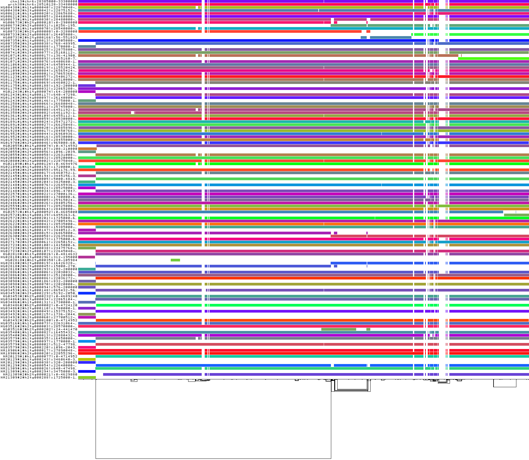
The complex region to the right side of the visualization corresponds to the MHC class II genes.

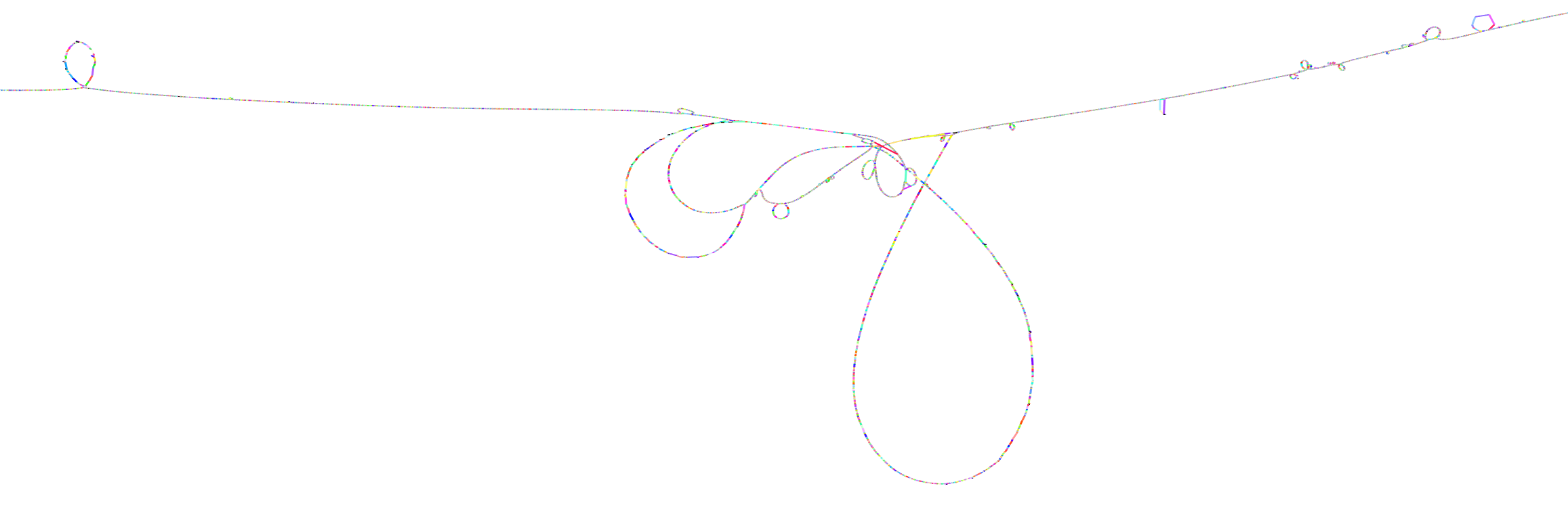
We can visualize this too, with gfaestus. The orientation and order are very similar to the above 1D visualization, letting us see how the graph looks in 2D.

Here, the splines we see correspond to sequences in the graph. Each node has a specific color, leading to the rainbow patterns that we see. Each change in color thus indicates a new allele in the pangenome.

Zooming in on the MHC class II genes shows a very complex structure. This is one of the most highly-diverged regions in the human genome. Balancing selection drives diversity here, as the genes in the MHC encode for features of the immune system. It is very advantageous for the human population to not have the same alleles here, so that our response to pathogens varies and it is not easy for a single pathogen to cause illness in all people.

Finally, we can get a compressed mode output from odgi viz which shows us a kind of heatmap across the graph space. For the full MHC graph, this is very boring: we have coverage almost everywhere:

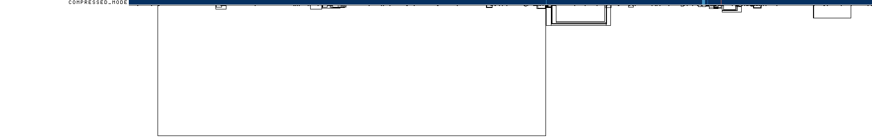
We’ll use this when making privvg transformations of the graph to get a sense of what we lose with different parameter combinations.

odgi priv provides the primary interface to apply the privvg algorithm to a graph.

Here we extract a haplotype sample of 10kbp sequences, targeting 100x total coverage, and emitting a progress message:

We see that there are ~53k paths in the graph with a similar step count to our input graph, so the paths are much more fragmented. The compressed mode heatmap is very similar to our full graph.

Let’s try to get longer haplotypes, say 50kbp.

And 100kbp:

Huge holes have shown up in the view! This means that there are parts of the graph which we were not able to sample. The cause is straightforward: these regions do not contain any exactly shared haplotypes of 100kbp. Thus, our haplotype frequency filter odgi priv -c 2 is preventing us from seeing any of them. This indicates that for us to obtain a differentially private synthetic pangenome with very long haplotypes across the MHC, we will need to have many more individuals in the input pangenome. With more individuals, we would expect a higher chance that a group of them has the exact same haplotype across one of these dropout loci.

Of course, haplotypes of even 10kbp are very useful. And for practical purposes, even 1kbp is a reasonable length for many downstream analyses. The practical utility of a differentially private pangenome is high in the MHC, so long as we can sample shorter haplotypes. The MHC represents one of the most extreme cases in the pangenome in terms of diversity and low rates of haplotype identity. This suggests that it should be straightforward to build a differentially private pangenome from the draft human pangenome!

One parameter defines how noisy our transformation is: \(\epsilon\). A low \(\epsilon\) is likely to be private, but we may introduce too much noise for the database to be useful. So we want to consider changing this parameter and looking at its effect on the output.

When \(\epsilon\) is small, it means that it is difficult for an adversary to distinguish, for pairs of adjacent databases, the database which includes or does not include an individual. In other words, \(\epsilon\) defines the degree of noise, noisy sampling, or blurring that is added to differentially private queries or synthetic databases. When the amount of noise is large (when \(\epsilon\) is small), it overwhelms the effects of addition or subtraction of a single individual, thus making it impossible for the adversary to distinguish individuals in general [dwork2014].

Let’s sweep \(\epsilon\) and look at a population genetic parameter of the output graph, the allele frequency. In our graphs, allele frequency is equivalent to path depth over nodes (which in the pangenome variation graph are sequences, which are equivalent to alleles). We can extract it with odgi depth -d and plot it with R.

The input allele/node frequency spectrum shows a sharp peak at ~90, which is the number of haplotypes in the pangenome.

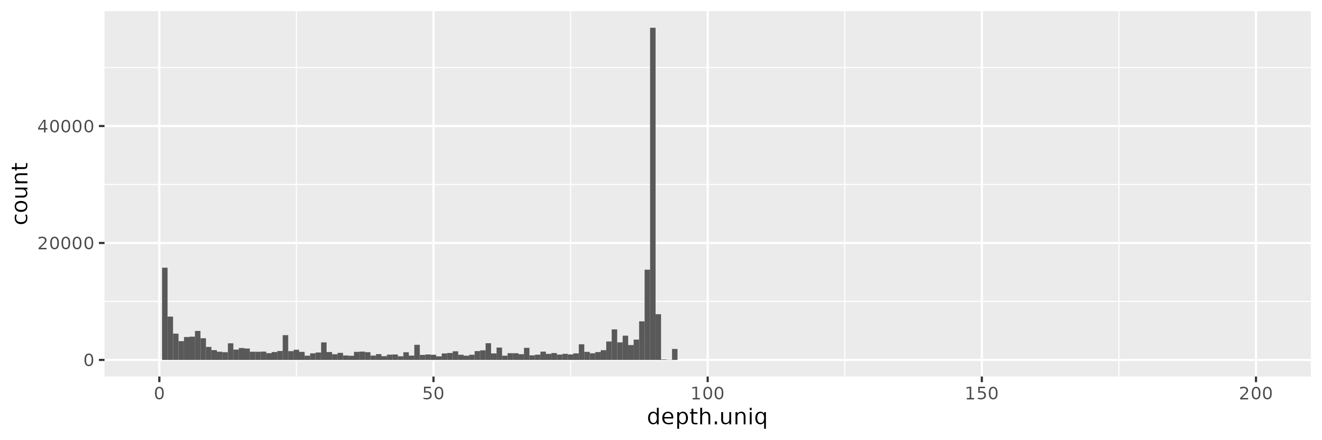
But we do not see a similar pattern in a 100x-sampled privvg when using a small \(\epsilon = 0.001\). We actually see a rather flat frequency distribution, which hides the peaks seen in the real data:

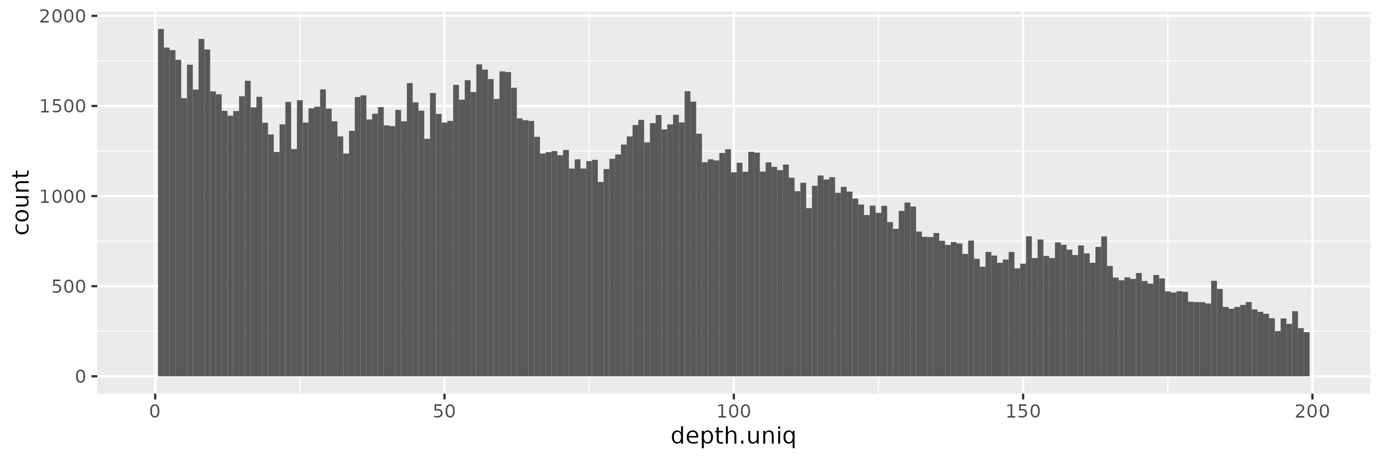
The pattern is similar for \(\epsilon = 0.01\):

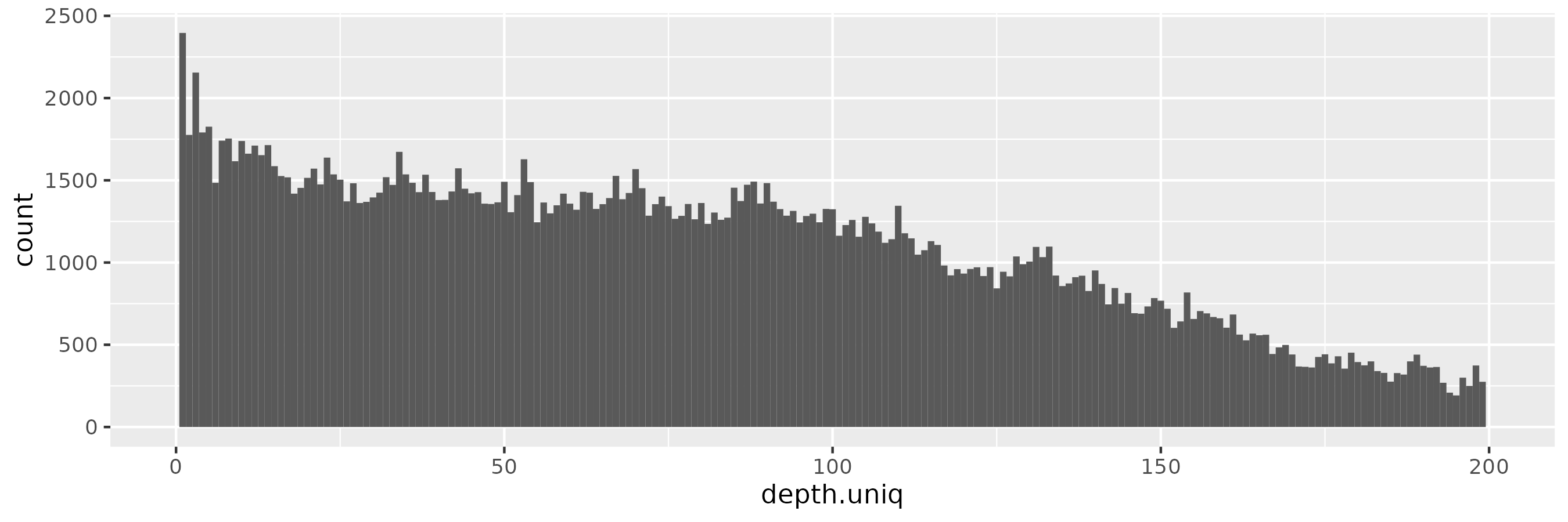
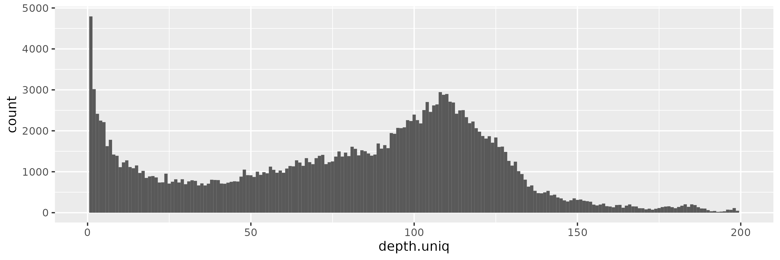
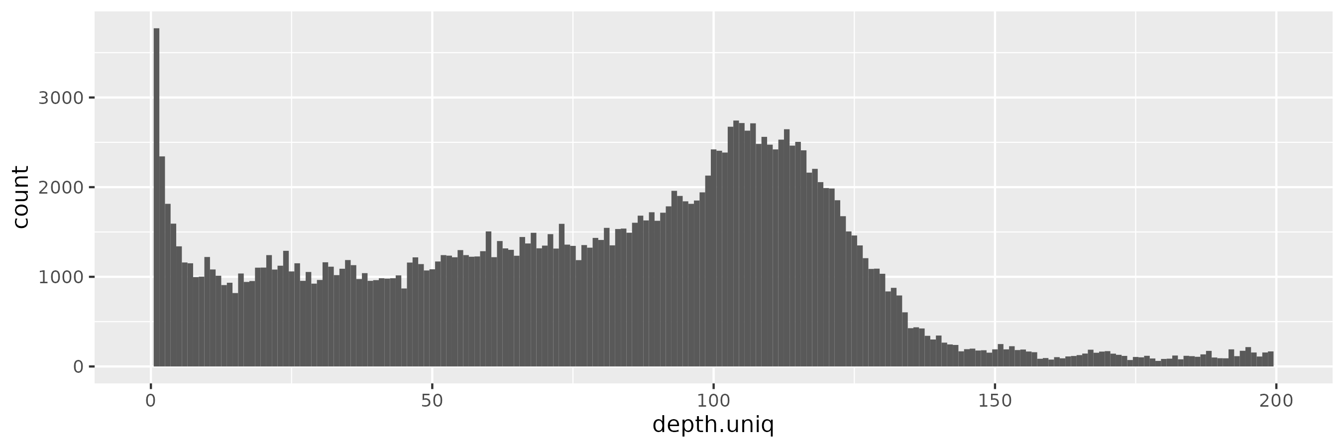
At \(\epsilon = 0.1\), we start to observe more low-frequency alleles, consistent with a more relaxed privacy guarantee:

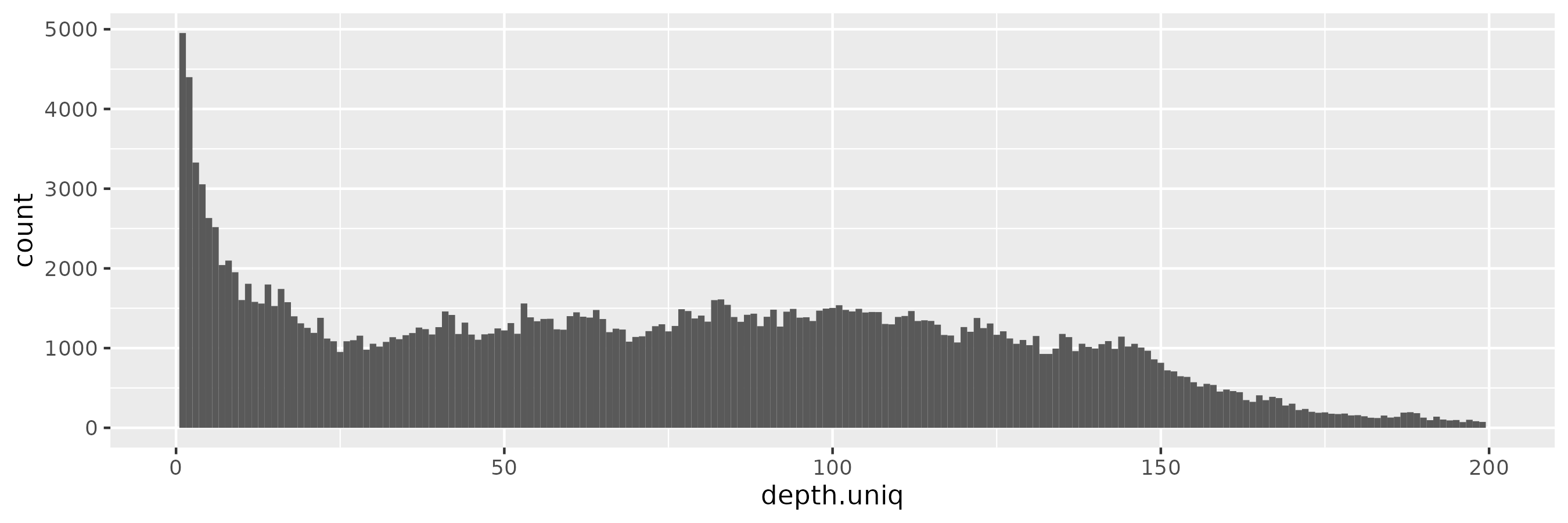
And with \(\epsilon = 1\), we begin to see a peak around the target depth (100x):

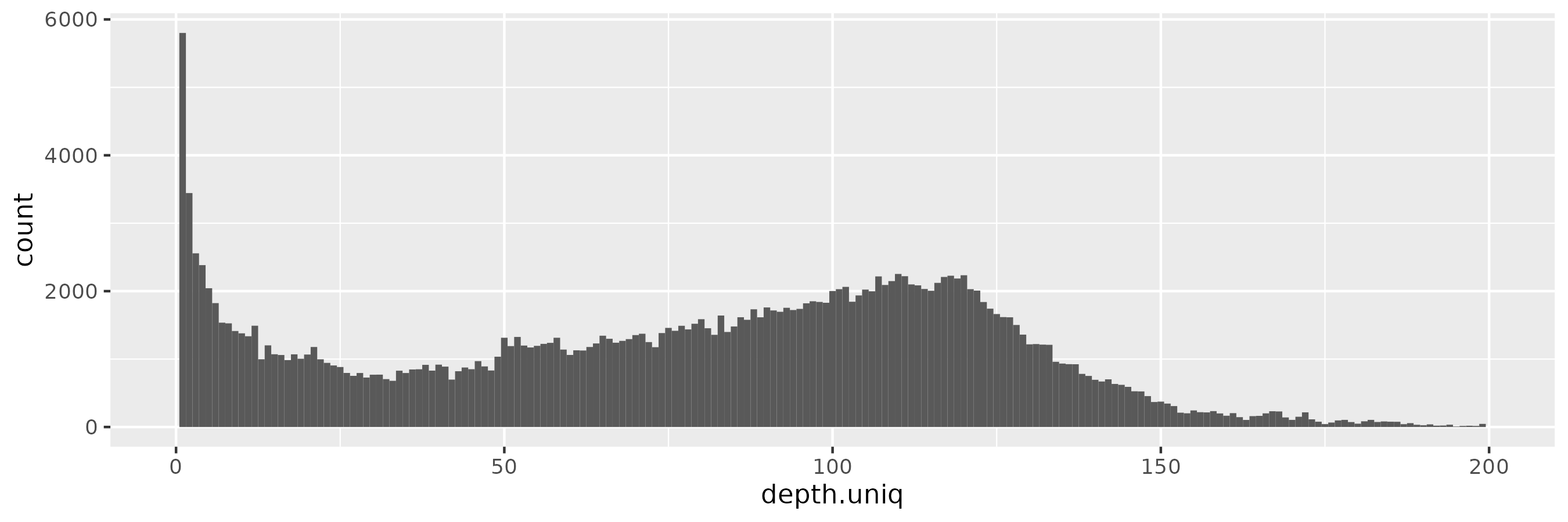
This becomes progressively more prononced as we increase \(\epsilon = 10\):

And for \(\epsilon = 100\), the pattern is starting to be reminiscient of the kind of distribution we saw in the input data, with the peak near 100x rather than 90x of course:

By increasing \(\epsilon\) we are exponentially down-weighting rare haplotypes. We don’t follow them because the weight of a given option, \(\exp(\epsilon u(x, r) / \Delta u)\), becomes exponentially larger with higher utility (a.k.a. log1p(haplotype_frequency)). In effect, we often run down the graph sampling the major allele at every site. The sampled haplotypes can become very long and uniform in length, because they tend to always match our minimum frequency threshold requirements and run to our target length.

At the same time, when increasing \(\epsilon\), we observe an increase in rare alleles in the privvg synthetic pangenome. This pattern is consistent with a reduction in differential privacy guarantees. Rare alleles support the identification of individuals.

These patterns gives the impression that \(\epsilon\) is behaving as expected, although it’s worth noting that the interaction between our utility function and privacy is also somewhat confusing. We will already tend to over-weight common haplotypes due to them having greater utility by our definition.

We plan to close the project with two final deliverables that build on our implementation.

First, we will develop a privvg model from the HPRCy1 draft pangenome. We will apply methods like the assembled genomes compressor agc to measure the effect of different parameters on the whole pangenome behavior of privvg. Because the HPRC is fully public, the utility of this resource is merely research-related, but it will be the first attempt to build such a model for a whole collection of completely assembled genomes.

Second, we will establish a set of synthetic "pangenome pairs", where we add and remove specific individuals. We will present these as a public competition, with a nominal prize for anyone who is able to determine which individuals have been removed from which pangenome model. By soliciting empirically-driven responses and workflows that describe the privacy-adversarial attacks, we will build practice around the problem of differential privacy on pangenomes. In effect, this will attach a bounty on the quality of our approach, initating a long-running audit that will establish the practical foundation for applying privvg to real cohort data.